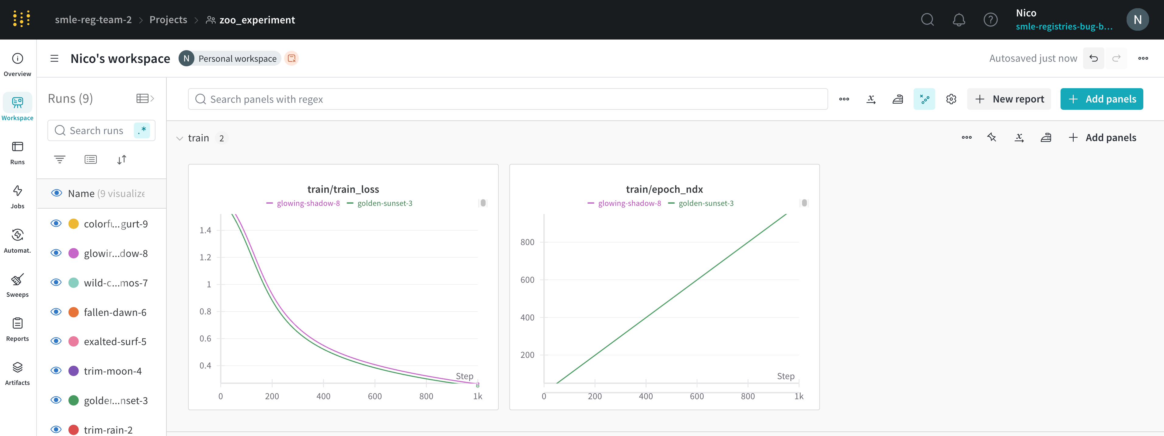
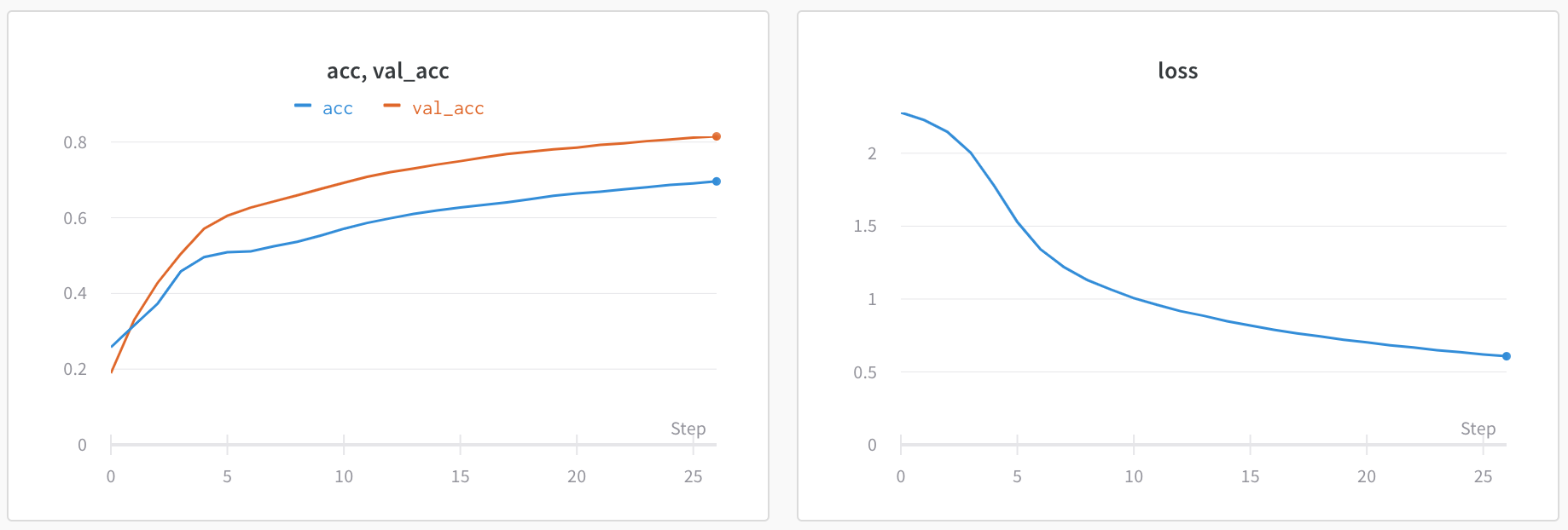
Line plots show up by default when you plot metrics over time with wandb.Run.log(). Customize with chart settings to compare multiple lines on the same plot, calculate custom axes, and rename labels.
Edit line plot settings
This section shows how to edit the settings for an individual line plot panel, all line plot panels in a section, or all line plot panels in a workspace.
wandb.Run.log() that you use to log the y-axis.Individual line plot
A line plot’s individual settings override the line plot settings for the section or the workspace. To customize a line plot:
- Hover your mouse over the panel, then click the gear icon.
- Within the drawer that appears, select a tab to edit its settings.
- Click Apply.
Line plot settings
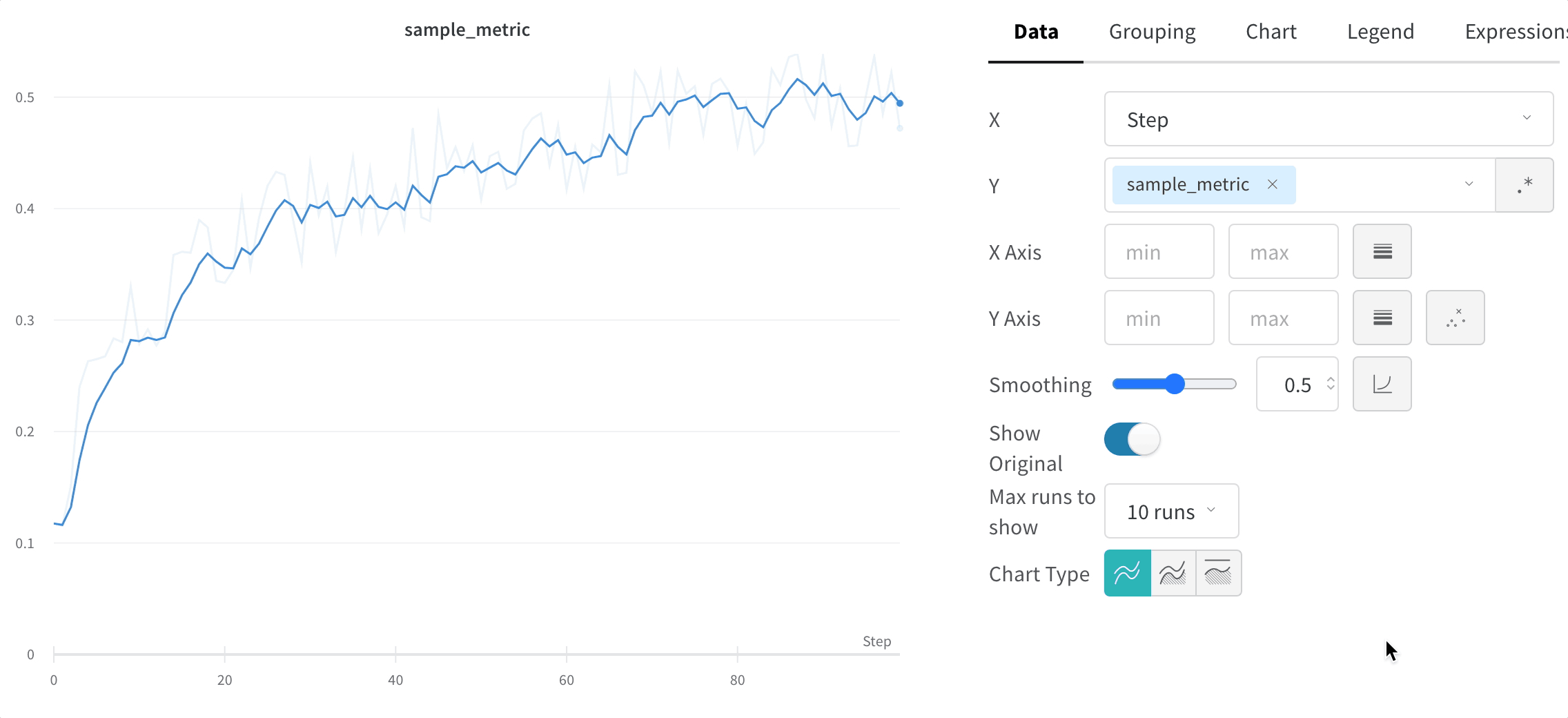
You can configure these settings for a line plot:
Date: Configure the plot’s data-display details.
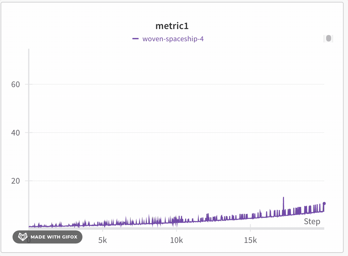
- X axis: Select the value to use for the X axis (defaults to Step). You can change the x-axis to Relative Time or select a custom axis based on values you log with W&B. You can also configure the X axis scale and range.
- Relative Time (Wall) is clock time since the process started, so if you started a run and resumed it a day later and logged something that would be plotted a 24hrs.
- Relative Time (Process) is time inside the running process, so if you started a run and ran for 10 seconds and resumed a day later that point would be plotted at 10s.
- Wall Time is minutes elapsed since the start of the first run on the graph.
- Step increments by default each time
wandb.Run.log()is called, and is supposed to reflect the number of training steps you’ve logged from your model.
- Y axis: Select one or more y-axes from the logged values, including metrics and hyperparameters that change over time. You can also configure the X axis scale and range.
- Point aggregation method. Either Random sampling (the default) or Full fidelity. Refer to Sampling.
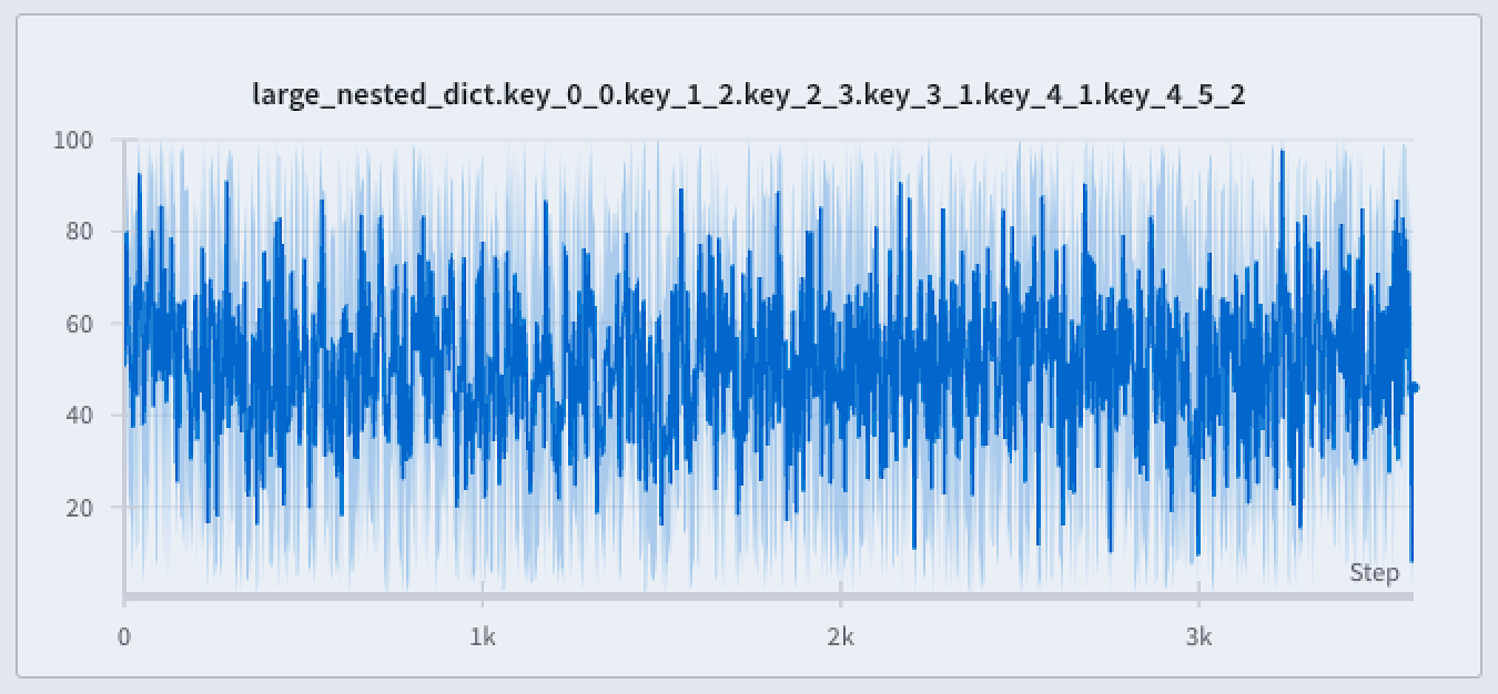
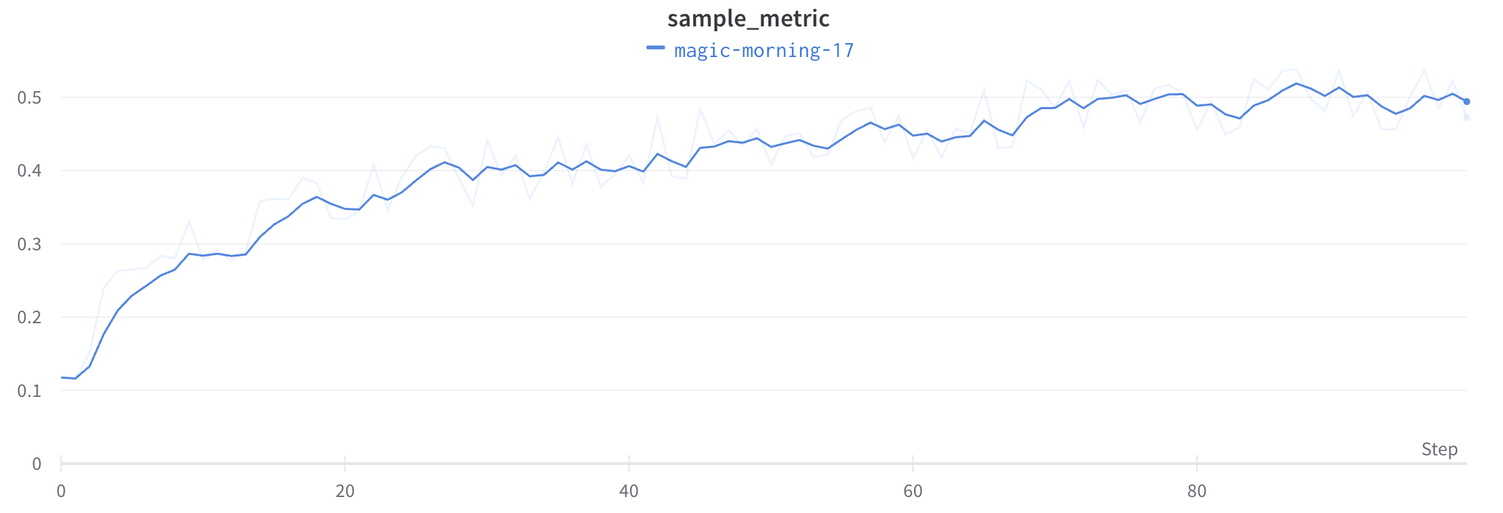
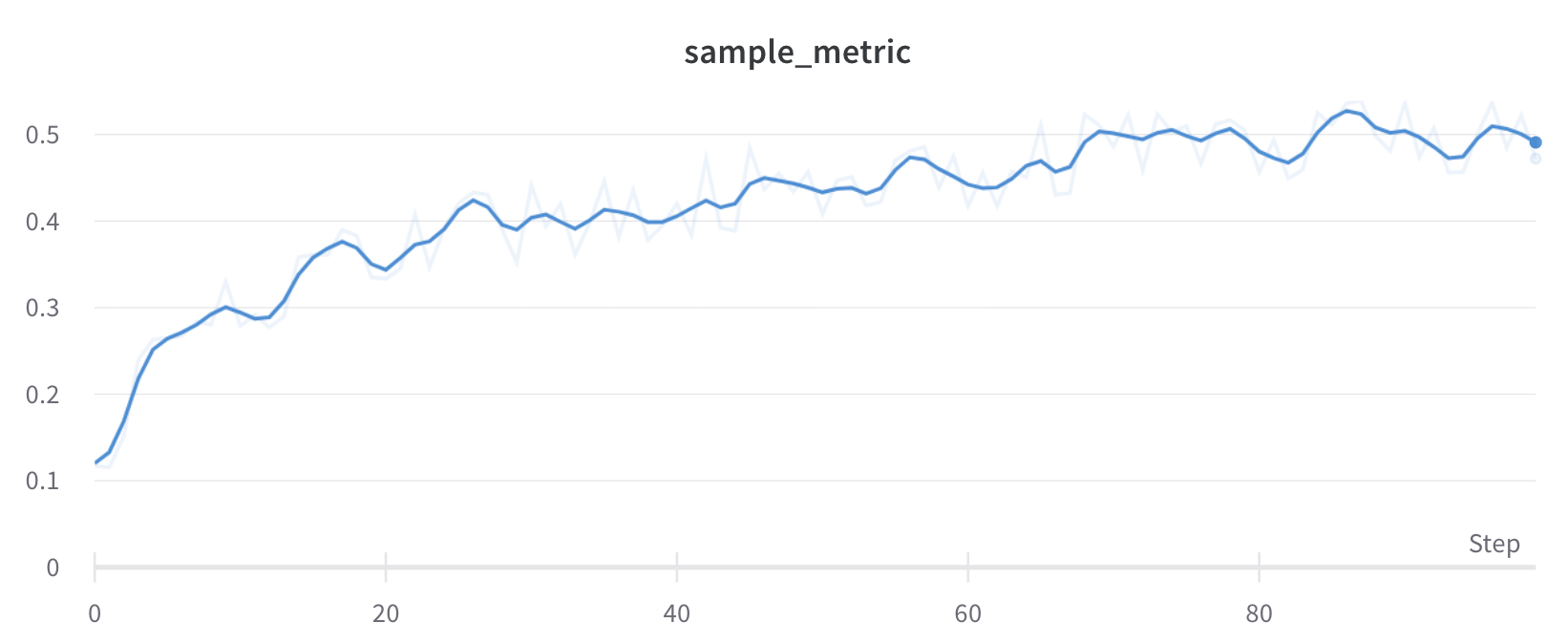
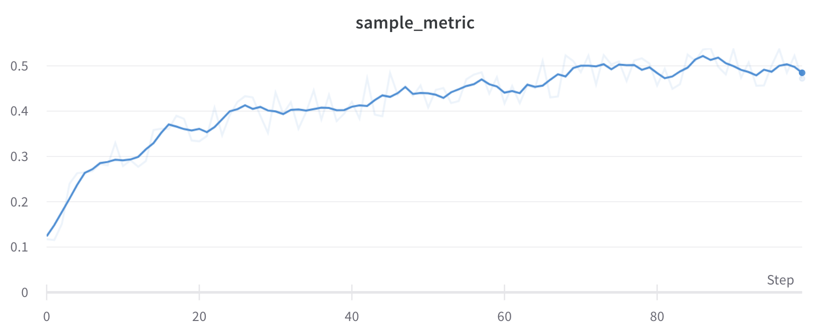
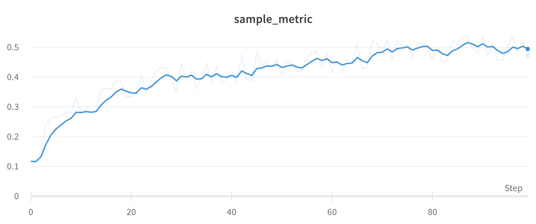
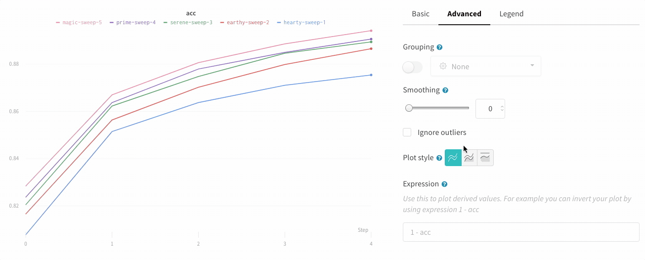
- Smoothing: Change the smoothing on the line plot. Defaults to Time weighted EMA. Other values include No smoothing, Running average, and Gaussian.
- Outliers: Rescale to exclude outliers from the default plot min and max scale.
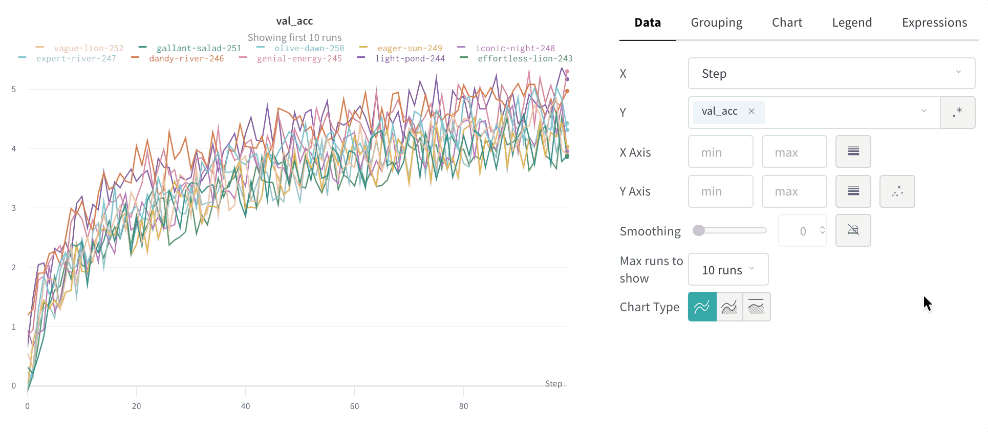
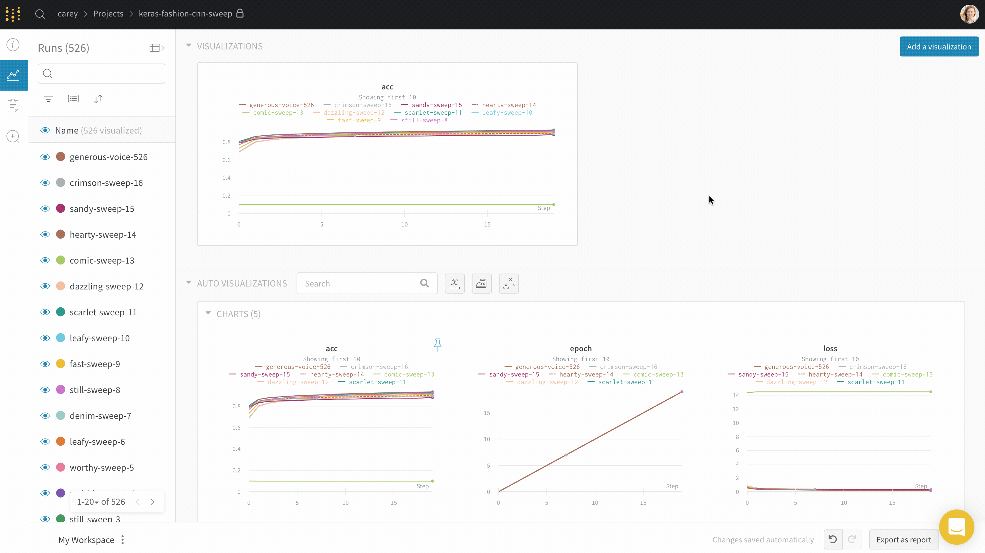
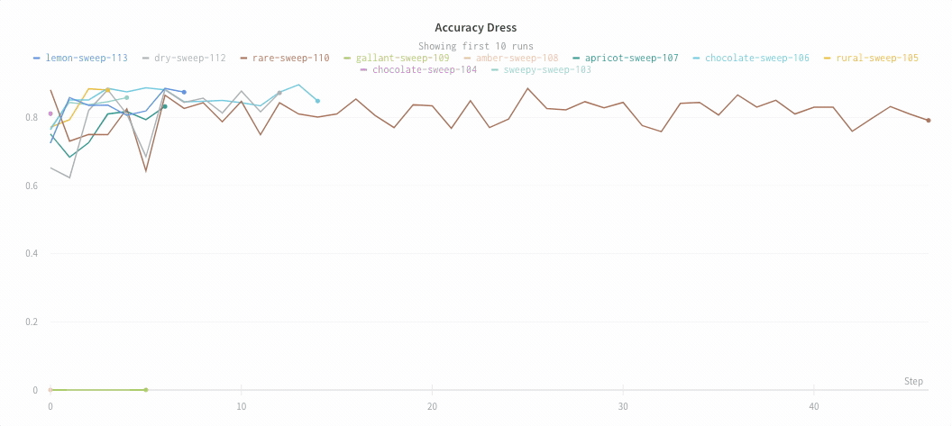
- Max number of runs or groups: Show more lines on the line plot at once by increasing this number, which defaults to 10 runs. You’ll see the message “Showing first 10 runs” on the top of the chart if there are more than 10 runs available but the chart is constraining the number visible.
- Chart type: Change between a line plot, an area plot, and a percentage area plot.
Grouping: Configure whether and how to group and aggregate runs in the plot.
- Group by: Select a column, and all the runs with the same value in that column will be grouped together.
- Agg: Aggregation— the value of the line on the graph. The options are mean, median, min, and max of the group.
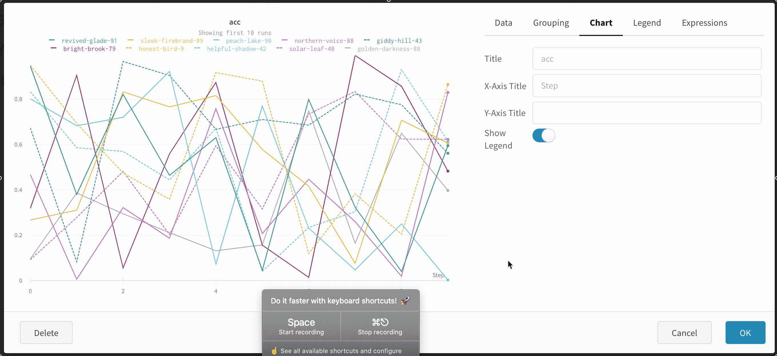
Chart: Specify titles for the panel, the X axis, and the Y axis, and the -axis, hide or show the legend, and configure its position.
Legend: Customize the appearance of the panel’s legend, if it is enabled.
- Legend: The field in the legend for each line in the plot in the legend of the plot for each line.
- Legend template: Define a fully customizable template for the legend, specifying exactly what text and variables you want to show up in the template at the top of the line plot as well as the legend that appears when you hover your mouse over the plot.
Expressions: Add custom calculated expressions to the panel.
- Y Axis Expressions: Add calculated metrics to your graph. You can use any of the logged metrics as well as configuration values like hyperparameters to calculate custom lines.
- X Axis Expressions: Rescale the x-axis to use calculated values using custom expressions. Useful variables include**_step** for the default x-axis, and the syntax for referencing summary values is
${summary:value}
All line plots in a section
To customize the default settings for all line plots in a section, overriding workspace settings for line plots:
- Click the section’s gear icon to open its settings.
- Within the drawer that appears, select the Data or Display preferences tabs to configure the default settings for the section. For details about each Data setting, refer to the preceding section, Individual line plot. For details about each display preference, refer to Configure section layout.
All line plots in a workspace
To customize the default settings for all line plots in a workspace:
- Click the workspace’s settings, which has a gear with the label Settings.
- Click Line plots.
- Within the drawer that appears, select the Data or Display preferences tabs to configure the default settings for the workspace.
-
For details about each Data setting, refer to the preceding section, Individual line plot.
-
For details about each Display preferences section, refer to Workspace display preferences. At the workspace level, you can configure the default Zooming behavior for line plots. This setting controls whether to synchronize zooming across line plots with a matching x-axis key. Disabled by default.
-
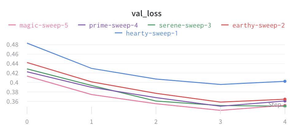
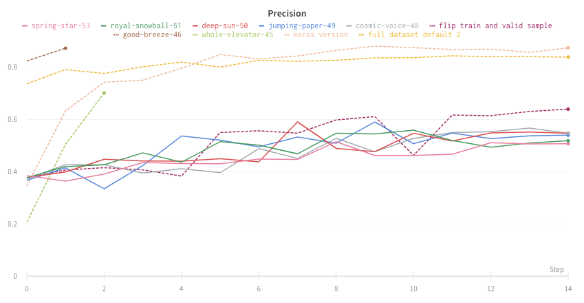
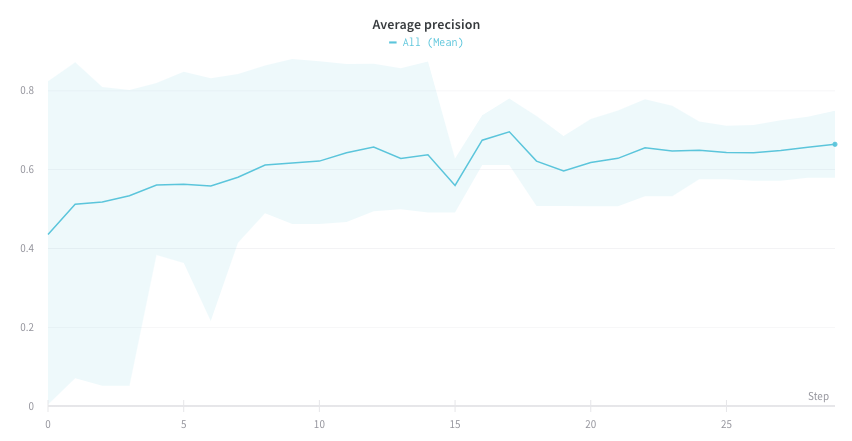
Visualize average values on a plot
If you have several different experiments and you’d like to see the average of their values on a plot, you can use the Grouping feature in the table. Click “Group” above the run table and select “All” to show averaged values in your graphs.
Here is what the graph looks like before averaging:
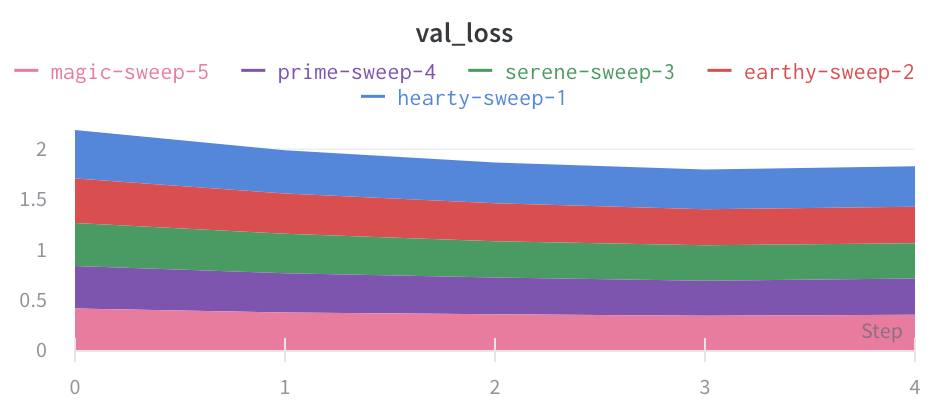
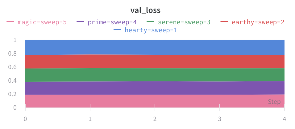
The proceeding image shows a graph that represents average values across runs using grouped lines.
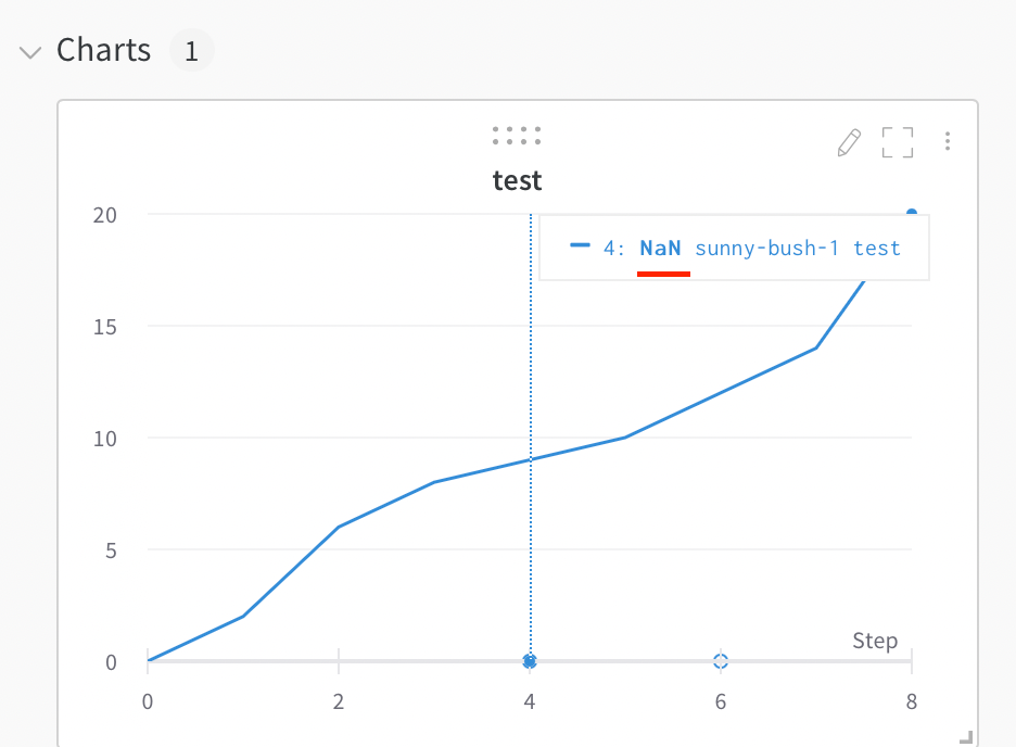
Visualize NaN value on a plot
You can also plot NaN values including PyTorch tensors on a line plot with wandb.Run.log(). For example:
with wandb.init() as run:
    # Log a NaN value
    run.log({"test": float("nan")})
Compare two metrics on one chart
- Select the Add panels button in the top right corner of the page.
- From the left panel that appears, expand the Evaluation dropdown.
- Select Run comparer
Change the color of the line plots
Sometimes the default color of runs is not helpful for comparison. To help overcome this, wandb provides two instances with which one can manually change the colors.
Each run is given a random color by default upon initialization.
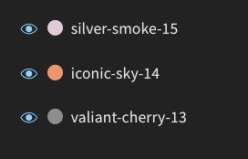
Upon clicking any of the colors, a color palette appears from which we can manually choose the color we want.
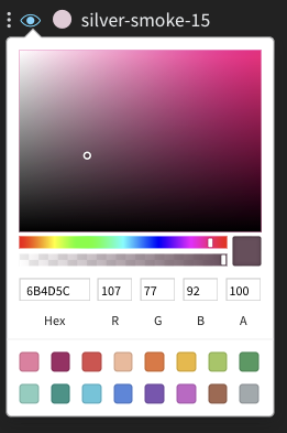
- Hover your mouse over the panel you want to edit its settings for.
- Select the pencil icon that appears.
- Choose the Legend tab.
Visualize on different x axes
If you’d like to see the absolute time that an experiment has taken, or see what day an experiment ran, you can switch the x axis. Here’s an example of switching from steps to relative time and then to wall time.
Area plots
In the line plot settings, in the advanced tab, click on different plot styles to get an area plot or a percentage area plot.
Zoom
Click and drag a rectangle to zoom vertically and horizontally at the same time. This changes the x-axis and y-axis zoom.
Hide chart legend
Turn off the legend in the line plot with this simple toggle:
Create a run metrics notification
Use Automations to notify your team when a run metric meets a condition you specify. An automation can post to a Slack channel or run a webhook.
From a line plot, you can quickly create a run metrics notification for the metric it shows:
- Hover over the panel, then click the bell icon.
- Configure the automation using the basic or advanced configuration controls. For example, apply a run filter to limit the scope of the automation, or configure an absolute threshold.
Learn more about Automations.
Visualize CoreWeave infrastructure alerts
Observe infrastructure alerts such as GPU failures, thermal violations, and more during machine learning experiments you log to W&B. During a W&B run, CoreWeave Mission Control monitors your compute infrastructure.
If an error occurs, CoreWeave sends that information to W&B. W&B populates infrastructure information onto your run’s plots in your project’s workspace. CoreWeave attempts to automatically resolve some issues, and W&B surfaces that information in the run’s page.
Find infrastructure issues in a run
W&B surfaces both SLURM job issues and cluster node issues. View infrastructure errors in a run:
- Navigate to your project on the W&B App.
- Select the Workspace tab to view your project’s workspace.
- Search and select the name of the run that contains an infrastructure issue. If CoreWeave detected an infrastructure issue, one or more red vertical lines with an exclamation mark overlay the run’s plots.
- Select an issue on a plot or select the Issues button in the top right of the page. A drawer appears that lists each issue reported by CoreWeave.
Tip
To views runs with infrastructure issues at a glance, pin the Issues column to your W&B Workspace to view runs that logged an issue at a glance. For more information about how to pin a column, see Customize how runs are displayed.The Overall Grafana view at the top of the drawer redirects you to the SLURM job’s Grafana dashboard, which contains system-level details about the run. The Issues summary describes the root error that the SLURM job reported to CoreWeave Mission Control. The summary section also describes any attempts to automatically resolve the error made by CoreWeave.
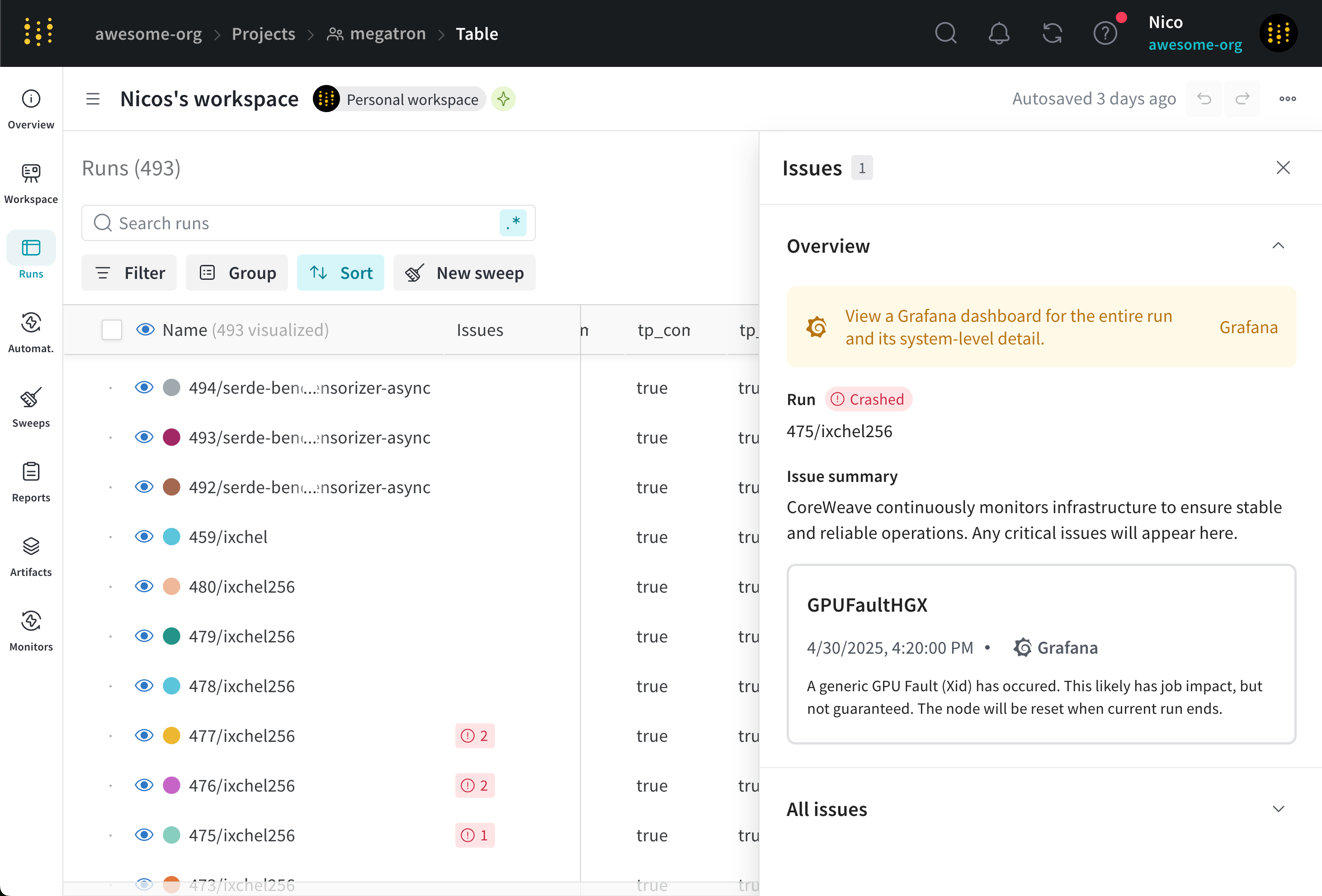
The All Issues list all issues that occurs during the run in chronological order, with the most recent issue at the top. The list contains the job issue and node issue alerts. Within each issue alert is the name of the issue, the timestamp when the issue occurred, a link to the Grafana dashboard for that issue, and a brief summary that describes the issue.
The following table shows example alerts for each category of infrastructure issues:
| Category | Example alerts |
|---|---|
| Node Availability & Readiness | KubeNodeNotReadyHGX, NodeExtendedDownTime |
| GPU/Accelerator Errors | GPUFallenOffBusHGX, GPUFaultHGX, NodeTooFewGPUs |
| Hardware Errors | HardwareErrorFatal, NodeRAIDMemberDegraded |
| Networking & DNS | NodeDNSFailureHGX, NodeEthFlappingLegacyNonGPU |
| Power, Cooling, and Management | NodeCPUHZThrottle, RedfishDown |
| DPU & NVSwitch | DPUNcoreVersionBelowDesired, NVSwitchFaultHGX |
| Miscellaneous | NodePCISpeedRootGBT, NodePCIWidthRootSMC |
For detailed information on error types, see the SLURM Job Metrics on the CoreWeave Docs.
Debug infrastructure issues
Each run that you create in W&B corresponds to a single SLURM job in CoreWeave. You can view a failed job’s Grafana dashboard or discover more information about a single node. The link within the Overview section of the Issues drawer links to the SLURM job Grafana dashboard. Expand the All Issues dropdown to view both job and node issues and their respective Grafana dashboards.
Note
The Grafana dashboard is only available for W&B users with a CoreWeave account. Contact W&B to configure Grafana with your W&B organization.Depending on the issue, you may need to adjust the SLURM job configuration, investigate the node’s status, restart the job, or take other actions as needed.
For more information about CoreWeave SLURM jobs in Grafana, see Slurm/Job Metrics on the CoreWeave Docs. See Job info: alerts for detailed information about job alerts.